In recent years, light fields have become a major research topic and their applications span across the entire spectrum of classical image processing. Among the different methods used to capture a light field are the lenslet cameras, such as those developed by Lytro. While these cameras give a lot of freedom to the user, they also create light field views that suffer from a number of artefacts. As a result, it is common to ignore a significant subset of these views when doing high-level light field processing. We propose a pipeline to process light field views, first with an enhanced processing of RAW images to extract sub-aperture images, then a colour correction process using a recent colour transfer algorithm, and finally a denoising process using a state of the art light field denoising approach. We show that our method improves the light field quality on many levels, by reducing ghosting artefacts and noise, as well as retrieving more accurate and homogeneous colours across the sub-aperture images.
Implementation
All of our code is now available here (please cite the appropriate papers if you use or adapt these codes in your work):
RAW data decoding
Recolouring
Denoising
Datasets
Many of the Light Field datasets we processed are available for direct use in clean form here. Please cite our paper “A Pipeline for Lenslet Light Field Quality Enhancement”, ICIP 2018, if you use any of these data in you work. Two versions are available, without or with our denoising step :
Dataset (without denoising)
Dataset (with denoising)
Related publications
Sorry, no publications matched your criteria.
Additional results
Our pipeline was applied on a subset of the freely available EPFL1 and INRIA2 datasets.
Successful colour correction
|
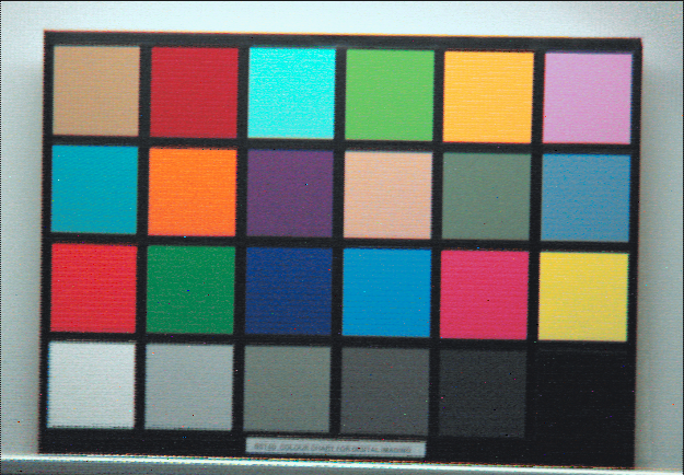
Centre view (palette) |
Original external view |
‘Centre’ recolouring |
‘Prop’ recolouring |
‘Prop+centre’ reco |
| Ankylosaurus_and_ Diplodocus_11 |
 |
 |
 |
 |
 |
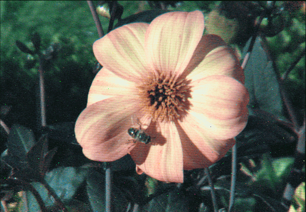
| Bee_12 |
 |
 |
 |
 |
 |
| Bee_22 |
 |
 |
 |
 |
 |
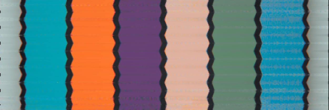
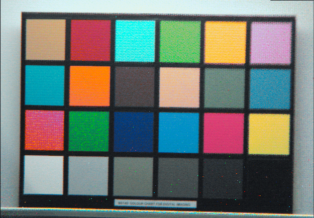
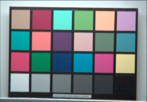
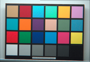
| Color_Chart_11 |
 |
 |
 |
 |
 |
| ChezEdgar2 |
 |
 |
 |
 |
 |
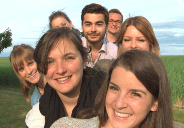
| Friends_11 |
 |
 |
 |
 |
 |
| Fruits2 |
 |
 |
 |
 |
 |
| Magnets_11 |
 |
 |
 |
 |
 |
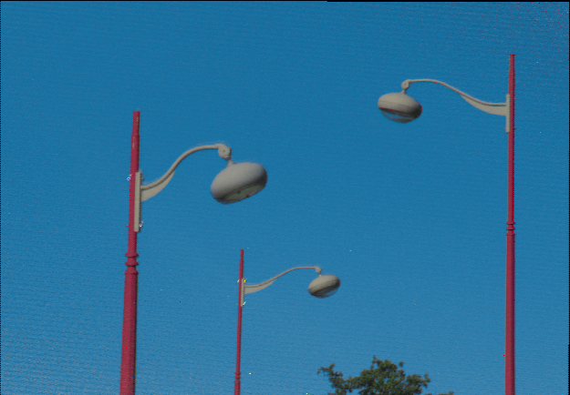
| Posts2 |
 |
 |
 |
 |
 |
| Rose2 |
 |
 |
 |
 |
 |
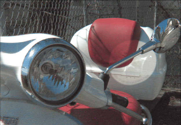
| Vespa1 |
 |
 |
 |
 |
 |
Video examples
Left side : our decoding; right side : our recolouring (Bee_22).
Left side : our recolouring; right side : our denoising (Bee_22).
Left side : our decoding; right side : our recolouring (Color_Chart_11).
Left side : our recolouring; right side : our denoising (Color_Chart_11).
Epipolar images
Horizontal epipolar images.
|
Dansereau decoding |
Our pipeline (‘centre’) |
Our pipeline (‘prop’) |
Our pipeline (‘p+c’) |
| Bee_12 |
 |
 |
 |
 |
| Bee_22 |
 |
 |
 |
 |
| Color_Chart_11 |
 |
 |
 |
 |
| Fruits2 |
 |
 |
 |
 |
| Magnets_11 |
 |
 |
 |
 |
Vertical epipolar images.
|
Dansereau decoding |
Our pipeline (‘centre’) |
Our pipeline (‘prop’) |
Our pipeline (‘p+c’) |
| Bee_12 |
 |
 |
 |
 |
| Bee_22 |
 |
 |
 |
 |
| Color_Chart_11 |
 |
 |
 |
 |
| Fruits2 |
 |
 |
 |
 |
| Magnets_11 |
 |
 |
 |
 |
Fail cases
‘Centre’ recolouring scheme fail cases. First picture is the centre view (palette), the rest are fail cases (different views in the light field). (Color_Chart_11 dataset)
 |
 |
 |
 |
 |
 |
Examples of tiny details not being registered properly during colour correction. First picture is the centre view (palette), second is a fail case (neighbouring view of the centre one). (Posts2 dataset)
 |
 |
Recolouring fail cases when extreme specular effects are present. First picture is the centre view (palette), the rest are fail cases (different views in the light field). (Vespa1 dataset)
 |
 |
 |
Detailed metric results
Table 1 – Average recolouring results using PSNR. Higher values are better.
|
Decoded |
Prop |
Centre |
Prop+centre |
| Ankylosaurus_and_Diplodocus_11 |
29.2905 |
30.4249 |
30.1865 |
30.3422 |
| Bee_12 |
22.5770 |
24.0342 |
23.8479 |
23.9856 |
| Bee_22 |
20.7177 |
21.7383 |
21.5678 |
21.6599 |
| ChezEdgar2 |
25.8484 |
26.7639 |
26.7429 |
26.7728 |
| Color_Chart_11 |
21.0754 |
21.9253 |
21.6420 |
21.9139 |
| Friends_11 |
26.9947 |
27.3831 |
27.2762 |
27.3273 |
| Fruits2 |
21.0893 |
21.5367 |
21.4133 |
21.4574 |
| Magnets_11 |
27.8008 |
28.4443 |
28.3576 |
28.4102 |
| Posts2 |
25.4259 |
29.3566 |
28.8164 |
29.2133 |
Table 2 – Average recolouring results using SSIM. Higher values are better.
|
Decoded |
Prop |
Centre |
Prop+centre |
| Ankylosaurus_and_Diplodocus_11 |
0.9049 |
0.9324 |
0.9300 |
0.9317 |
| Bee_12 |
0.6550 |
0.7212 |
0.7099 |
0.7191 |
| Bee_22 |
0.5790 |
0.6156 |
0.6101 |
0.6135 |
| ChezEdgar2 |
0.9058 |
0.9152 |
0.9166 |
0.9162 |
| Color_Chart_11 |
0.8023 |
0.8165 |
0.8057 |
0.8170 |
| Friends_11 |
0.9239 |
0.9299 |
0.9290 |
0.9297 |
| Fruits2 |
0.6317 |
0.6379 |
0.6369 |
0.6375 |
| Magnets_11 |
0.9106 |
0.9346 |
0.9330 |
0.9348 |
| Posts2 |
0.8054 |
0.8659 |
0.8560 |
0.8637 |
Table 3 – Average recolouring results using S-CIELab. Lower values are better.
|
Decoded |
Prop |
Centre |
Prop+centre |
| Ankylosaurus_and_Diplodocus_11 |
11.6821 |
7.2841 |
7.3169 |
7.2584 |
| Bee_12 |
47.9358 |
33.7399 |
34.8856 |
33.8488 |
| Bee_22 |
62.2390 |
58.6591 |
57.2721 |
57.9372 |
| ChezEdgar2 |
29.2363 |
21.7885 |
21.0047 |
21.2967 |
| Color_Chart_11 |
36.2238 |
24.2762 |
26.1732 |
24.0729 |
| Friends_11 |
13.5950 |
11.5322 |
11.0613 |
11.2397 |
| Fruits2 |
47.8697 |
46.9557 |
44.3578 |
45.0527 |
| Magnets_11 |
15.0985 |
11.0375 |
10.7007 |
10.7644 |
| Posts2 |
23.6692 |
9.1165 |
9.9985 |
9.2863 |
Table 4 – Average recolouring results using CID. Lower values are better.
|
Decoded |
Prop |
Centre |
Prop+centre |
| Ankylosaurus_and_Diplodocus_11 |
0.4394 |
0.2110 |
0.1993 |
0.2071 |
| Bee_12 |
0.4277 |
0.2245 |
0.2210 |
0.2223 |
| Bee_22 |
0.5007 |
0.4455 |
0.4433 |
0.4413 |
| ChezEdgar2 |
0.2260 |
0.2253 |
0.2201 |
0.2210 |
| Color_Chart_11 |
0.4059 |
0.3869 |
0.3966 |
0.3876 |
| Friends_11 |
0.1266 |
0.1141 |
0.1128 |
0.1130 |
| Fruits2 |
0.3110 |
0.3049 |
0.3004 |
0.3007 |
| Magnets_11 |
0.5034 |
0.3056 |
0.3113 |
0.3112 |
| Posts2 |
0.0222 |
0.0216 |
0.0244 |
0.0228 |
Table 5 – Average recolouring results using Histogram distance. Lower values are better.
|
Decoded |
Prop |
Centre |
Prop+centre |
| Ankylosaurus_and_Diplodocus_11 |
0.3068 |
0.1583 |
0.1591 |
0.1597 |
| Bee_12 |
0.3419 |
0.2037 |
0.2153 |
0.2045 |
| Bee_22 |
0.2354 |
0.2238 |
0.1841 |
0.2039 |
| ChezEdgar2 |
0.2189 |
0.1225 |
0.1234 |
0.1234 |
| Color_Chart_11 |
0.2274 |
0.1540 |
0.1588 |
0.1536 |
| Friends_11 |
0.1928 |
0.1185 |
0.1170 |
0.1179 |
| Fruits2 |
0.1930 |
0.1669 |
0.1375 |
0.1482 |
| Magnets_11 |
0.2768 |
0.1545 |
0.1424 |
0.1497 |
| Posts2 |
0.4981 |
0.2388 |
0.2384 |
0.2437 |
Table 6 – Average noise level before and after denoising. Lower values are better.
|
Decoded |
Prop |
Prop+denoising |
Centre |
Centre+denoising |
Prop+centre+denoising |
| Ankylosaurus_and_Diplodocus_11 |
1.268 |
0.830 |
0.010 |
0.847 |
0.013 |
0.816 |
0.009 |
| Bee_12 |
3.019 |
2.132 |
0.262 |
2.362 |
0.345 |
2.160 |
0.262 |
| Bee_22 |
1.994 |
1.704 |
0.197 |
1.971 |
0.214 |
1.775 |
0.196 |
| ChezEdgar2 |
1.532 |
1.365 |
0.252 |
1.415 |
0.259 |
1.372 |
0.253 |
| Color_Chart_11 |
1.294 |
1.239 |
0.090 |
1.386 |
0.130 |
1.248 |
0.090 |
| Friends_11 |
0.584 |
0.563 |
0.110 |
0.570 |
0.105 |
0.586 |
0.113 |
| Fruits2 |
1.293 |
1.220 |
0.159 |
1.383 |
0.168 |
1.321 |
0.164 |
| Magnets_11 |
1.196 |
0.812 |
0.008 |
0.890 |
0.021 |
0.825 |
0.011 |
| Posts2 |
1.622 |
0.956 |
0.008 |
1.092 |
0.022 |
0.956 |
0.008 |
References
[1] M. Rerabek and T. Ebrahimi, “New Light Field Image Dataset”, in Proc. QoMEX, 2016.
[2] “Inria lytro illum dataset”, http://www.irisa.fr/temics/demos/lightField/CLIM/DataSoftware.html.